How I Built CloudFront Log Analytics for $3,300/Year

  Published on December 30, 2025

Observability platforms charge per gigabyte. CloudFront logs? That adds up. Here’s how I built analytics for a nearly fixed $275/month using ClickHouse Cloud: percentiles, dashboards, and full control.

This takes us into the “walk” part of the crawl-walk-run framework that I have established in earlier posts. This is characterized by log volume growing and the need to ask more holistic questions. We know the site is up, but how is it performing for our users? What unwanted traffic patterns (attacks) exist? By the end of this post you will have some techniques for building visualizations as well. Yes, I’ll talk about tools I like too.

SMART Goals: AWS CloudFront Analysis

Let’s scope this project down with a favorite tool of mine, SMART goals.

• Specific: Setup log analytics powerful enough to monitor latency in percentiles of our web presence as reported by AWS CloudFront logs.
• Measurable: Watch costs of the solution.
• Achievable: I have Flu-B and am only working at half speed.
• Relevant: Build foundations for understanding how to create powerful logging Observability platforms on the cheap.
• Time Bound: Doable in hours.

This isn’t a general solution to logging Observability. This also isn’t a solution for an instant page if the site is down. The goal is to ask more holistic questions and show how I think of the fundamentals of how I view Observability problems.

Flow and Design

Architecture

I have AWS CloudFront legacy logging enabled via infrastructure as code (IaC). There are several CloudFront distributions and they send logs to the same S3 bucket using a prefix. Basically, code words for the various sites I have.

• cloudfront/pag
• cloudfront/app
• cloudfront/cardinality

From S3 the logs flow into ClickHouse Cloud. I don’t want to run and manage a complicated database, but I do want to use it.

Finally, let’s use a number of tools to visualize the data so we can see how to test the solution, use it in a one-off analysis problem solving manner, and build a dashboard of it.

Costs

A primary concern is avoiding network costs. Especially with logs, these can be quite significant. The ClickHouse Cloud instance will be in the same region as the S3 bucket. Rather than streaming the data to the instance I will use the S3Queue table engine to poll and consume data from S3 via API. CloudFront doesn’t charge to deposit the logs in S3, and with the ClickHouse Cloud instance in AWS in the same region they are not incurring charges by reading from the S3 bucket.

I have life cycle policies created in S3 and in ClickHouse to only keep the last 90 days worth of data. So I’m storing the data twice in this setup. S3 charges $0.023 per gig-month, and ClickHouse Cloud charges $0.025 per gig-month. In an enterprise setup I’d likely use S3 -> Glacier as cold long term storage and keep only a limited amount in ClickHouse for hot/warm queriable data. Or I could use my S3 bucket with a short retention for a staging area only as ClickHouse stores data in S3 as well and provides backups.

The primary cost is that of running the ClickHouse Cloud instance. For an 8GiB instance this is about $220 USD per month. Data queried over the SQL API will cause network egress charges, but I assume this to be very low compared to the amount of data going into the ClickHouse Cloud instance.

Let’s be generous and say costs are $275 USD per month. That’s a $3,300 per year Observability solution. This serves a data volume of about 2TiB compressed or likely about 14 TiB uncompressed. Not bad.

Tradeoffs

The S3Queue table engine introduces latency into the ingestion pipeline and this is my tradeoff for keeping costs lower. The polling is tunable but I prefer fewer LIST API hits against S3. 30s polling is roughly $0.43 USD per month of LIST requests and ClickHouse has dynamic polling, so this is worst case.

The AWS CloudFront documentation states:

CloudFront delivers logs for a distribution up to several times an hour. In general, a log file contains information about the requests that CloudFront received during a given time period. CloudFront usually delivers the log file for that time period to your destination within an hour of the events that appear in the log. Note, however, that some or all log file entries for a time period can sometimes be delayed by up to 24 hours.

This makes the tradeoff nearly moot as ClickHouse will have better latency guarantees than AWS CloudFront log delivery. In fact polling at 30s intervals is aggressive.

Implementation

Enable Log Delivery

This is up to how your IaC works. Take note of what region the S3 bucket is created in. This should be the same region as the ClickHouse Cloud instance for optimum costing.

AWS IAM Roles

This took the longest time for me. As many times as I’ve done cross account IAM Roles you would think this would get less frustrating. Never does.

The ClickHouse Cloud instance will run as an AWS IAM Role listed in Settings -> Network Security Information. Find that in your ClickHouse Cloud console for the instance in question. We will allow that IAM Role to assume a new IAM Role in our AWS account. That new role will have access to read the S3 bucket. See Accessing S3 Data Securely.

Use your IaC to create a new AWS IAM Role. The trust policy will trust the foreign IAM Role (the one the ClickHouse instance runs as) to assume this new role.

 1
 2
 3
 4
 5
 6
 7
 8
 9
10
11
12
13
14
15
16
17
18
19
20
21
22
23
24

# Trust policy allowing ClickHouse service role to assume this role
data "aws_iam_policy_document" "clickhouse_assume_role" {
  statement {
    effect = "Allow"

    principals {
      type        = "AWS"
      identifiers = [var.clickhouse_role_arn]
    }

    actions = ["sts:AssumeRole"]
  }
}

# IAM role that ClickHouse will assume
resource "aws_iam_role" "clickhouse_access" {
  name               = "ClickHouseAccess-${local.Environment}"
  assume_role_policy = data.aws_iam_policy_document.clickhouse_assume_role.json

  tags = {
    Name        = "ClickHouse S3 Logs Access"
    Environment = local.Environment
  }
}

Attach to your new AWS IAM Role a policy allowing it to read from the S3 bucket containing the CloudFront logs.

 1
 2
 3
 4
 5
 6
 7
 8
 9
10
11
12
13
14
15
16
17
18
19
20
21
22
23
24
25
26
27
28
29
30

# IAM policy granting S3 read permissions for logs bucket
data "aws_iam_policy_document" "clickhouse_s3_access" {
  # Allow getting bucket location and listing bucket
  statement {
    effect = "Allow"

    actions = [
      "s3:GetBucketLocation",
      "s3:ListBucket",
    ]

    resources = [
      aws_s3_bucket.logs.arn,
    ]
  }

  # Allow reading objects from the bucket
  statement {
    effect = "Allow"

    actions = [
      "s3:Get*",
      "s3:List*",
    ]

    resources = [
      "${aws_s3_bucket.logs.arn}/*",
    ]
  }
}

When the S3Queue table is built we will tell ClickHouse what AWS IAM Role to assume by giving in the ARN of the IAM Role in our account.

1
2
3
4
5
6

ENGINE = S3Queue(
    'https://<BUCKET_NAME>.s3.<REGION>.amazonaws.com/cloudfront/**.gz',
    'TabSeparated',
    'gzip',
    extra_credentials(role_arn = 'arn:aws:iam::012345678901:role/ClickHouseAccess-foobar')
)

Schema

SQL is pronounced “squeal” because that’s the sound you make when you use it.

That was my old adage. But today we have AI and ClickHouse provides really reasonable documentation. Which means creating the schema needed to handle this data is just magically easy. Ok, yes, I did have to yell at Claude to use Float64 instead of Float32 types, but other than that the produced schema was really spot on.

The S3Queue table engine concept has 3 distinct parts.

1. The Queue: A table that you cannot select from as it reads data only once. This specifies where in S3 and what format the files are.
2. The Destination Table: A normal table of data in your desired format/types. This is a partitioned table to manage data aging and volume.
3. The Materialized View: This object triggers the Queue to read in data, then the materialized view reformats the data as needed and inserts it into the destination table. Want to URL decode all the paths? This is where you do that.

The schema that I used is here: cloudfront-clickhouse-schema.sql.

Interesting points:

• This partitions by month where I would recommend by day.
• mode='ordered' can potentially skip late arriving files.

Debugging

The hardest bit was making sure that ClickHouse could read files out of S3. The detail being the difference between an access denied problem and a zero files found problem (when I misstyped the glob path). I used this SQL query to debug access problems. Again, thanks to AI for building this with the right table schema in it.

1
2
3
4
5
6
7
8

SELECT
  _path, _file
FROM s3(
  'https://s3.amazonaws.com/<BUCKET_NAME>/cloudfront/**.gz',
  'TabSeparated',
  'c_ip String, c_port String, cs_bytes String, cs_cookie String, cs_host String, cs_method String, cs_protocol String, cs_protocol_version String, cs_referer String, cs_uri_query String, cs_uri_stem String, cs_user_agent String, date String, fle_encrypted_fields String, fle_status String, sc_bytes String, sc_content_len String, sc_content_type String, sc_range_end String, sc_range_start String, sc_status String, ssl_cipher String, ssl_protocol String, time String, time_taken String, time_to_first_byte String, x_edge_detailed_result_type String, x_edge_location String, x_edge_request_id String, x_edge_response_result_type String, x_edge_result_type String, x_forwarded_for String, x_host_header String',
  'gzip',
  extra_credentials(role_arn = 'arn:aws:iam::012345678901:role/ClickHouseAccess-foobar'))

Putting Everything Together

We Have Data!

The ClickHouse Cloud console easily told me that my destination table cloudfront_logs had data in it. Now I could use my CLI based client to start testing.

SELECT
    sc_status AS code,
    quantile(0.5)(time_taken) AS p50,
    quantile(0.9)(time_taken) AS p90,
    quantile(0.99)(time_taken) AS p99
FROM cloudfront_logs
WHERE date = yesterday()
GROUP BY sc_status

Query id: 32aa8834-f1fd-4e05-ad44-0d63fe88b0ca

   ┌─code─┬────p50─┬─────────────────p90─┬──────────────────p99─┐
1. │  200 │ 0.1235 │              0.2558 │   0.4546500000000001 │
2. │  206 │  0.052 │               0.052 │                0.052 │
3. │  301 │      0 │                   0 │ 0.001569999999999993 │
4. │  302 │   0.19 │              0.2844 │  0.30563999999999997 │
5. │  304 │ 0.0655 │ 0.16230000000000003 │  0.19712999999999997 │
6. │  403 │  0.001 │               0.001 │                0.001 │
7. │  404 │  0.143 │               0.254 │              0.28654 │
   └──────┴────────┴─────────────────────┴──────────────────────┘

7 rows in set. Elapsed: 0.005 sec. Processed 2.07 thousand rows, 23.45 KB
(378.50 thousand rows/s., 4.28 MB/s.) Peak memory usage: 2.03 MiB.

That’s pretty much our goal. We can monitor today’s traffic latencies by status code.

CLI Charts

ClickHouse can do basic graphing for us at the CLI. It’s not pretty. It’s not what I would call a dashboard. But for testing and proof of concept – you bet! Let’s look at this over time for yesterday (UTC). The parameters of bar() set the min and max lengths of the produced bar chart.

SELECT
    toStartOfFifteenMinutes(timestamp) AS time_bucket,
    count() AS hits,
    bar(count(), 0, 1000, 50) AS chart
FROM cloudfront_logs
WHERE date = yesterday()
GROUP BY time_bucket
ORDER BY time_bucket ASC
FORMAT PrettyCompactMonoBlock

Query id: b9217671-4d92-4a02-9321-3ca5707c1623

    ┌─────────time_bucket─┬─hits─┬─chart────────────────┐
 1. │ 2025-12-29 21:00:00 │  398 │ ███████████████████▉ │
 2. │ 2025-12-29 21:15:00 │  128 │ ██████▍              │
 3. │ 2025-12-29 21:30:00 │   15 │ ▊                    │
 4. │ 2025-12-29 21:45:00 │   18 │ ▉                    │
 5. │ 2025-12-29 22:00:00 │   22 │ █                    │
 6. │ 2025-12-29 22:15:00 │   21 │ █                    │
 7. │ 2025-12-29 22:30:00 │  101 │ █████                │
 8. │ 2025-12-29 22:45:00 │   17 │ ▊                    │
 9. │ 2025-12-29 23:00:00 │    6 │ ▎                    │
10. │ 2025-12-29 23:15:00 │    7 │ ▎                    │
11. │ 2025-12-29 23:30:00 │    1 │                      │
12. │ 2025-12-29 23:45:00 │  107 │ █████▎               │
    └─────────────────────┴──────┴──────────────────────┘

12 rows in set. Elapsed: 0.005 sec. Processed 1.93 thousand rows, 19.30 KB (361.28 thousand rows/s., 3.61 MB/s.)
Peak memory usage: 654.30 KiB.

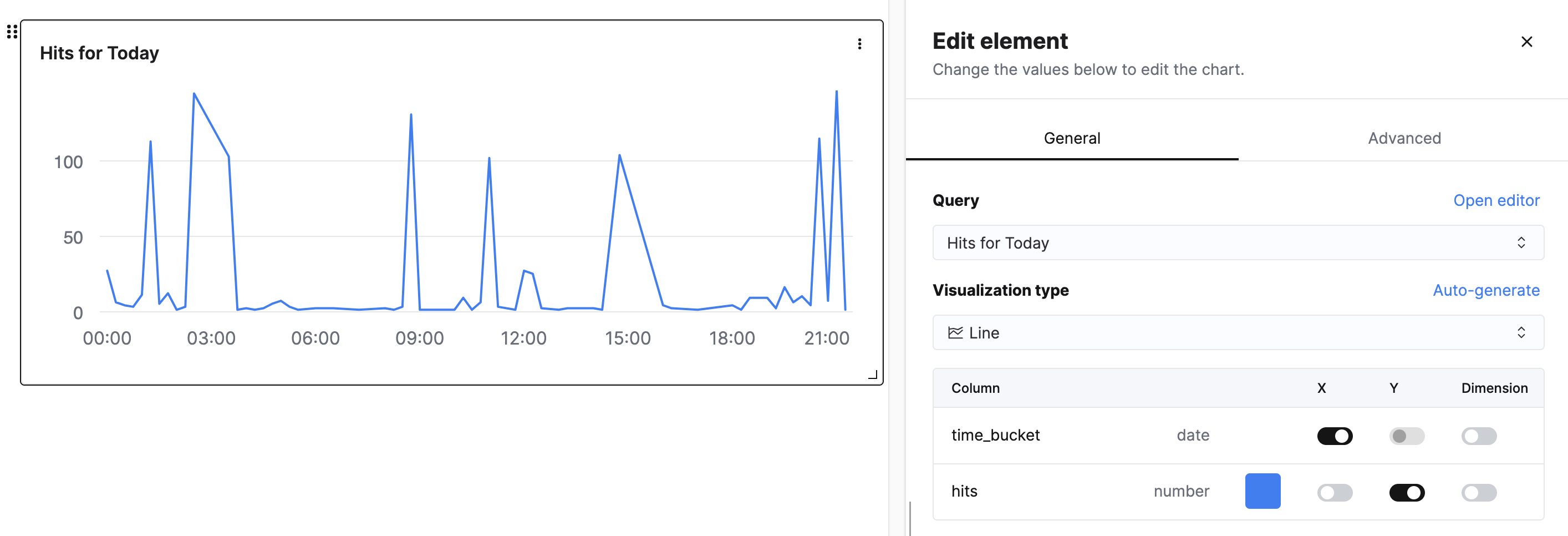
ClickHouse Cloud Console

The ClickHouse Cloud Console has some interesting (and fairly new) support for dashboards. It doesn’t appear to have Grafana’s style of picking random date ranges, but I’ve also found these useful.

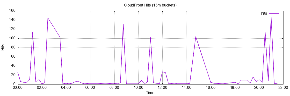
GNUPlot

GNUPlot has always had a soft place in my heart. It’s what many scientists and engineers still use to generate graphs in their papers.

$ clickhouse-client --query "
SELECT
    formatDateTime(toStartOfFifteenMinutes(timestamp), '%Y-%m-%dT%H:%i:%S') AS time_bucket,
    count() AS hits
FROM o11y.cloudfront_logs
WHERE date = today()
GROUP BY time_bucket
ORDER BY time_bucket ASC
FORMAT TabSeparated
" | gnuplot -e "
set terminal png size 1200,400;
set output 'hits.png';
set title 'CloudFront Hits (15m buckets)';
set xlabel 'Time';
set ylabel 'Hits';
set xdata time;
set timefmt '%Y-%m-%dT%H:%M:%S';
set format x '%H:%M';
set grid;
plot '-' using 1:2 with lines linewidth 2 title 'hits'
"

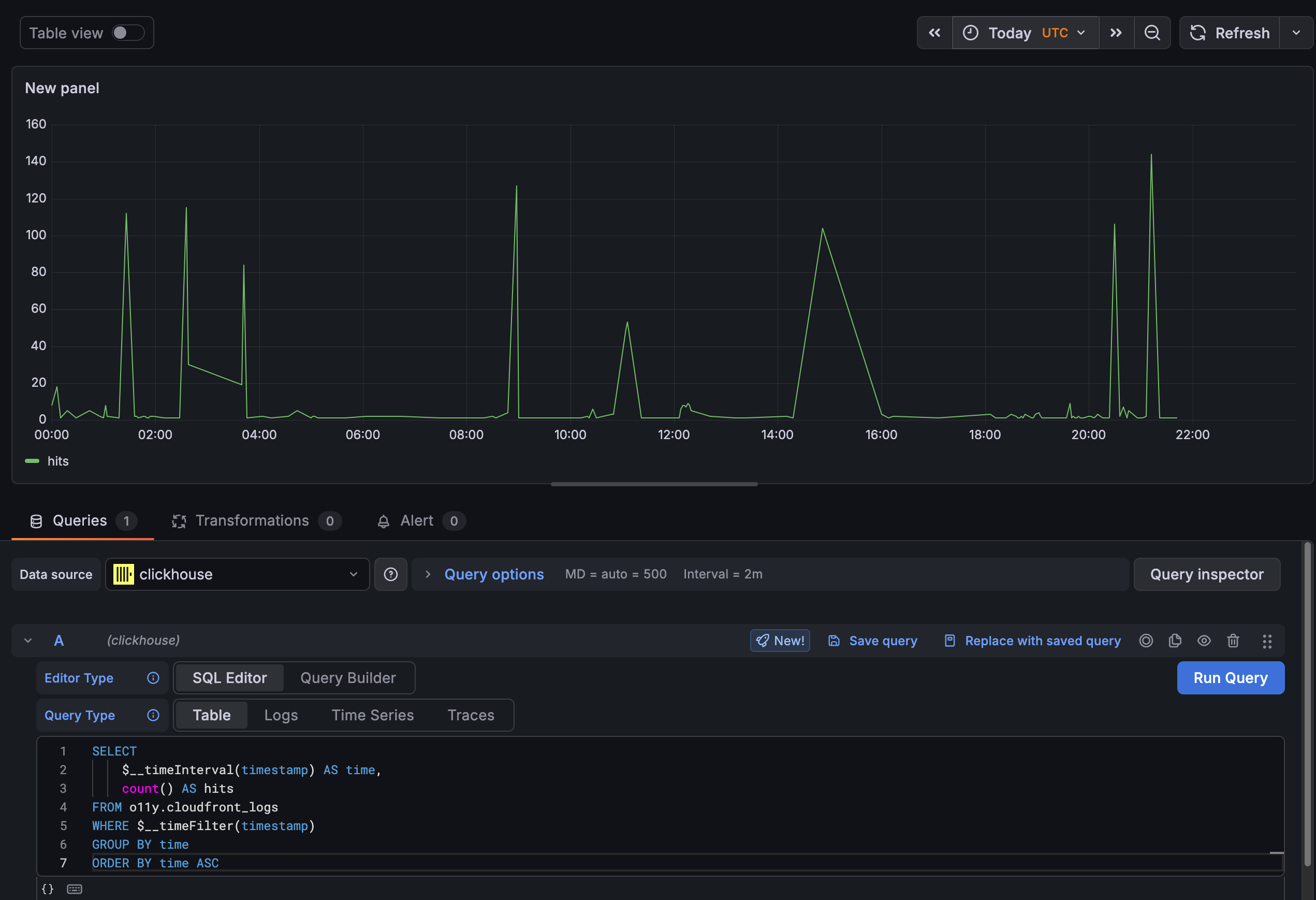
Grafana Cloud

Grafana has always been my Visualization platform of choice for Observability data. The key feature has always been the ability to zoom in and out of any time window and set my timezone. (I commonly set it to UTC as I did here to get this to align with the above graphs.) AI helped me with the SQL syntax again to integrate with the Grafana time picker.

Best of all, this is the free forever version of Grafana Cloud. So now you know how to use hosted Grafana for free. You’re welcome.

Wrapping Up

There you have it. An analytical powerhouse of a solution that can answer almost any question you can throw at CloudFront logs. Total costs are 4 figures per year even at reasonable scale. Compare that to a vendor charging you to ingest each line in your CloudFront logs.

The biggest obstacle to this type of work in the past has been mastering SQL. It’s not really a language, but a standard. Or at least it varies so much with each implementation I don’t think of it as a language. But we’ve used this tool to master data since the 1970s. So there is a unique power here. One that doesn’t become irrelevant whenever the next new shiny database comes out. Today, we have AI and a LOT of history and documentation about SQL. That means while you have to check AI’s work for Float32 data types, not knowing SQL just isn’t an excuse any more. The schema would have taken me hours to piece together – and now this entire demo project was completed in an afternoon.

Are you looking for a similar solution? Contact me today!